A virtual sensor in three steps
Three steps take you from the measurement file to a deployable model: select the channels, train, export. All three run in the same application on your own machine, without a Python environment and without measurement data leaving the company network.
Step 1: Load measurement data and select the channels
Open your recording (CSV, MAT, MDF/MF4 or TXT), or import a CAN or CAN FD trace (.asc or .blf) decoded against its signal database (.dbc). On opening, every channel is aligned to a shared time axis, so signals recorded at different rates line up from the first strip onwards.
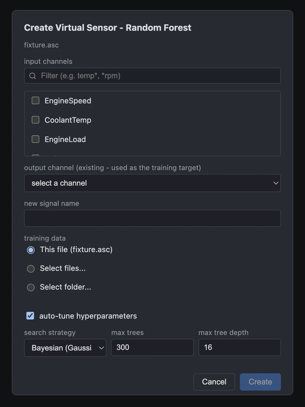
You then specify which channels the model receives as inputs and which signal it is to reproduce. Training data does not have to sit in a single file: alongside the current file, several files or an entire folder can be selected. Where the same physical signal is named differently across files, a mapping table assigns the correct channel per file once (reusable as a saved CSV file).
Step 2: Training and comparison
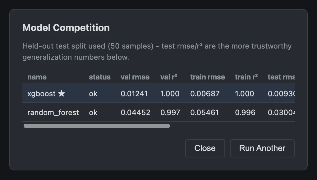
Random forest, XGBoost and neural networks are available. None of these families is the best for every task, so no preselection is required: Model Competition trains several candidates at once against the same input and output channels and sets them side by side in a leaderboard.
The accuracy of such surrogate models depends on hyperparameters, that is on parameters fixed before training: for a random forest, the number of trees, the maximum depth and the minimum leaf size; for a neural network, the number of layers, the neurons per layer and the learning rate. Data Sensors determines these hyperparameters automatically, by Bayesian optimisation, Random Search, Grid Search or a surrogate strategy.
Evaluation runs on a held-out validation split, that is on data the model in question was not trained on. The leaderboard lists validation RMSE and R² side by side, together with training time and a fit diagnosis. For sufficiently large data sets, a separate test split is set aside as well, used neither for training nor for model selection.
Step 3: Export as standalone code
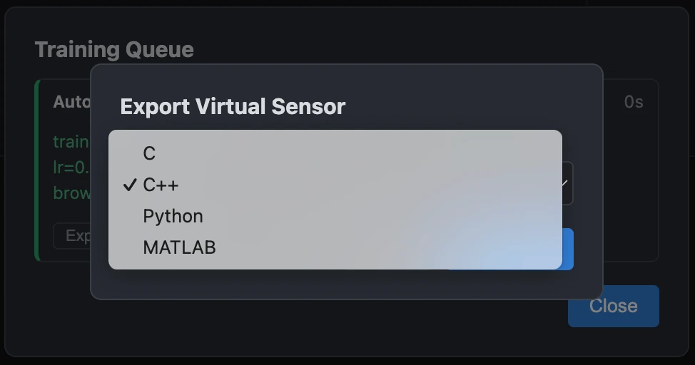
The selected model is exported directly to C, C++, Python or MATLAB: C for a plain MCU build, C++ for a class-based interface, Python for an analysis script or a service, MATLAB for use in a Simulink block. The generated code is a standalone implementation of the prediction function, with no dependency on Data Sensors and no runtime library to link against.
Export is either at full precision or int8-quantised, and the dialog shows an estimate of size and accuracy for both variants beforehand. The decision between flash budget and accuracy is therefore made before saving. Every leaderboard entry can be exported individually, not only the top one: a slightly less accurate model may run faster on your target hardware or fit the available memory better.
What you need for this
A measurement in which both the later input channels and the target quantity are recorded. The target quantity has to be measured with a physical sensor, since it serves as the reference for training. How much data is needed depends on the relationship; whether it was enough is shown by the evaluation on the held-out split. There are no further prerequisites: no Python installation, no account, no internet connection.